images.imfit
images.imfit contains three functions for fitting and value replacement.
Notes
For questions or comments please see our github page. We encourage and appreciate user feedback.
Most of these notebooks rely on basic knowledge of the Astropy FITS I/O module. If you are unfamiliar with this module please see the Astropy FITS I/O user documentation before using this documentation.
The fitting and replacement functionality of images.imfit can be replaced using tools available in Astropy and Scipy. Please see the linked doc pages for more details. These fitting functions have a lot more options and function types then what was available in IRAF.
All tasks in the images.imfit package provide the same function type options. Here is a conversion for these functions in Python:
- leg - astropy.modeling.polynomial.Legendre1D (or 2D)
- cheb - astropy.modeling.polynomial.Chebyshev1D (or 2D)
- spline1 - scipy.interpolate.UnivariantSpline
- spline3 - scipy.interpolate.CubicSpline
For ngrow the option (not covered here) see disk and dilation
from
skimage.morphology
Contents:
# Temporarily change default colormap to viridis
import matplotlib.pyplot as plt
plt.rcParams['image.cmap'] = 'viridis'
fit1d-lineclean
Please review the Notes section above before running any examples in this notebook
The fit1d task will fit a function to a 1d data array. The lineclean
task will take this same fitting tasks, and return your data array with
values outside a certain sigma limit replaced with the fitted values. We
can preform both these tasks with astropy and scipy functions.
You’ll find many more models defined in the astropy.models library
here
Below we show one example using a Legendre 1D fit, and another example using a linear spine. For the linear spline example we will go over an implementation of lineclean.
# Standard Imports
import numpy as np
from scipy.interpolate import UnivariateSpline

# Astronomy Specific Imports
from astropy.modeling import models, fitting, polynomial

# Plotting Imports/Setup
import matplotlib.pyplot as plt
%matplotlib inline
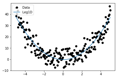
# Fitting - Legendre1D
# This example is taken in part from examples on the Astropy Modeling documentation

# Generate fake data
np.random.seed(0)
x = np.linspace(-5., 5., 200)
y = 0.5 * (3*x**2-1)
y += np.random.normal(0., 5, x.shape)

# Fit the data using the Legendre1D fitter
leg_init = polynomial.Legendre1D(2)
fit_leg = fitting.LevMarLSQFitter()
leg = fit_leg(leg_init, x, y)

# Plot solution
plt.plot(x, y, 'ko', label='Data')
plt.plot(x, leg(x), label='Leg1D')
plt.legend(loc=2)
WARNING: Model is linear in parameters; consider using linear fitting methods. [astropy.modeling.fitting]
<matplotlib.legend.Legend at 0x11a7a4908>
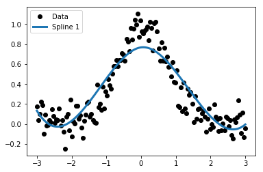
# Fitting - Spline1
# This example is taken in part from examples on the Astropy Modeling documentation

# Generate fake data
np.random.seed(0)
x = np.linspace(-3., 3., 150)
y = np.exp(-x**2) + 0.1 * np.random.randn(150)

# Fit the data using the Spline 1 fitter
spl1 = UnivariateSpline(x, y)
spl1.set_smoothing_factor(3)

# Plot solution
plt.plot(x, y, 'ko', label='Data')
plt.plot(x, spl1(x),lw=3,label='Spline 1')
plt.legend(loc=2)
<matplotlib.legend.Legend at 0x11a889b38>
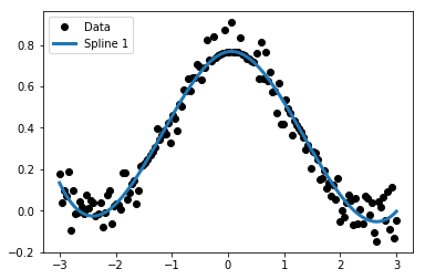
# Fitting and replacement of outlier values - Spline 1

# Fit array
fit_data = spl1(x)
residuals = fit_data-y
sigma = np.std(residuals)

# Let's reject everything outside of 1-sigma of the fit residuals
boolean_array = [np.absolute(residuals) > sigma]
y[boolean_array] = fit_data[boolean_array]
# Plot solution
plt.plot(x, y, 'ko', label='Data')
plt.plot(x, spl1(x),lw=3,label='Spline 1')
plt.legend(loc=2)
<matplotlib.legend.Legend at 0x11a9950f0>
imsurfit
Please review the Notes section above before running any examples in this notebook
Imsurfit has similiar functionality to the above tasks, but in 2
dimensions. Below we show a brief example, which can be extended as
shown above in the lineclean example. We use the
Polynomial2D astropy.modeling example here to showcase the usage
of models not found in this IRAF library.
# Standard Imports
import numpy as np

# Astronomy Specific Imports
from astropy.modeling import models, fitting

# Plotting Imports/Setup
import matplotlib.pyplot as plt
%matplotlib inline
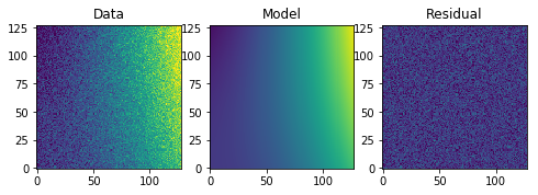
# Fitting - Polynomial2D
# This example is taken from the Astropy Modeling documentation

# Generate fake data
np.random.seed(0)
y, x = np.mgrid[:128, :128]
z = 2. * x ** 2 - 0.5 * y ** 2 + 1.5 * x * y - 1.
z += np.random.normal(0., 0.1, z.shape) * 50000.

# Fit the data using astropy.modeling
p_init = models.Polynomial2D(degree=2)
fit_p = fitting.LevMarLSQFitter()
p = fit_p(p_init, x, y, z)

# Plot the data with the best-fit model
plt.figure(figsize=(8, 2.5))
plt.subplot(1, 3, 1)
plt.imshow(z, origin='lower', interpolation='nearest', vmin=-1e4, vmax=5e4)
plt.title("Data")
plt.subplot(1, 3, 2)
plt.imshow(p(x, y), origin='lower', interpolation='nearest', vmin=-1e4,
           vmax=5e4)
plt.title("Model")
plt.subplot(1, 3, 3)
plt.imshow(z - p(x, y), origin='lower', interpolation='nearest', vmin=-1e4,
           vmax=5e4)
plt.title("Residual")
WARNING: Model is linear in parameters; consider using linear fitting methods. [astropy.modeling.fitting]
<matplotlib.text.Text at 0x119e94ac8>