images.imfilter
The images.imfilter IRAF package provides an assortment of image filtering and convolution tasks.
Notes
For questions or comments please see our github page. We encourage and appreciate user feedback.
Most of these notebooks rely on basic knowledge of the Astropy FITS I/O module. If you are unfamiliar with this module please see the Astropy FITS I/O user documentation before using this documentation.
Python replacements for the images.imfilter tasks can be found in the
Astropy and Scipy packages. Astropy convolution offers two convolution
options, convolve() is better for small kernels, and
convolve_fft() is better for larger kernels, please see the Astropy
convolution doc page
and Astropy Convolution How
to for
more details. For this notebook, we will use convolve. Check out the
list of kernels and filters avaialble for
Astropy,
and Scipy
Although astropy.convolution is built on scipy, it offers
several advantages: * can handle NaN values * improved options for
boundaries * provided built in kernels
So when possible, we will be using astropy.convolution functions in
this notebook. The ability to handle NaN values allows us to replicate
the behavior of the zloreject/zhireject parameter in the imfilter
package. See the rmedian entry for an example.
You can select from the following boundary rules in
astropy.convolution: * none * fill * wrap * extend
You can select from the following boundary rules in
scipy.ndimage.convolution: * reflect * constant * nearest *
mirror * wrap
Below we change the matplotlib colormap to viridis. This is
temporarily changing the colormap setting in the matplotlib rc file.
Important Note to Users: There are some differences in algorithms between some of the IRAF and Python Interpolations. Proceed with care if you are comparing prior IRAF results to Python results. For more details on this issue see the filed Github issue.
Contents:
# Temporarily change default colormap to viridis
import matplotlib.pyplot as plt
plt.rcParams['image.cmap'] = 'viridis'
boxcar
Please review the Notes section above before running any examples in this notebook
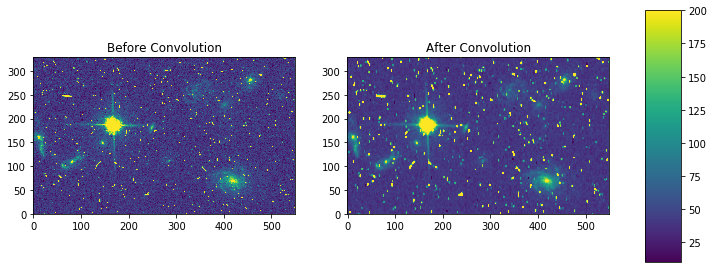
The boxcar convolution does a boxcar smoothing with a given box size,
and applies this running average to an array. Here we show a 2-D example
using Box2DKernel, which is convinient for square box sizes.
# Standard Imports
import numpy as np

# Astronomy Specific Imports
from astropy.io import fits
from astropy.convolution import convolve as ap_convolve
from astropy.convolution import Box2DKernel
from astroquery.mast import Observations

# Plotting Imports/Setup
import matplotlib.pyplot as plt
%matplotlib inline
# Download test file using astroquery, this only needs to be run once
# and can be skipped if using your own data.
# Astroquery will only download file if not already present.
obsid = '2004663553'
Observations.download_products(obsid,productFilename="jczgx1ppq_flc.fits")
INFO: Found cached file ./mastDownload/HST/JCZGX1PPQ/jczgx1ppq_flc.fits with expected size 167964480. [astroquery.query]
| Local Path | Status | Message | URL |
|---|---|---|---|
| str47 | str8 | object | object |
| ./mastDownload/HST/JCZGX1PPQ/jczgx1ppq_flc.fits | COMPLETE | None | None |
# grab subsection of fits images
test_data = './mastDownload/HST/JCZGX1PPQ/jczgx1ppq_flc.fits'
sci1 = fits.getdata(test_data,ext=1)
my_arr = sci1[700:1030,2250:2800]

# setup our kernel
box_kernel = Box2DKernel(3)
# perform convolution
result = ap_convolve(my_arr, box_kernel, normalize_kernel=True)
plt.imshow(box_kernel, interpolation='none', origin='lower')
plt.title('Kernel')
plt.colorbar()
plt.show()

fig, axes = plt.subplots(nrows=1, ncols=2)
pmin,pmax = 10, 200
a = axes[0].imshow(my_arr,interpolation='none', origin='lower',vmin=pmin, vmax=pmax)
axes[0].set_title('Before Convolution')
a = axes[1].imshow(result,interpolation='none', origin='lower',vmin=pmin, vmax=pmax)
axes[1].set_title('After Convolution')

fig.subplots_adjust(right = 0.8,left=0)
cbar_ax = fig.add_axes([0.85, 0.15, 0.05, 0.7])
fig.colorbar(a, cax=cbar_ax)
fig.set_size_inches(10,5)
plt.show()
convolve
Please review the Notes section above before running any examples in this notebook
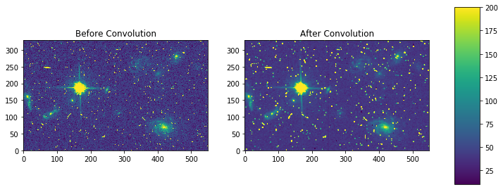
The convolve task allows you to convolve your data array with a kernel
of your own creation. Here we show a simple example of a rectangular
kernel applied to a 10 by 10 array using the
astropy.convolution.convolve function
# Standard Imports
import numpy as np

# Astronomy Specific Imports
from astropy.io import fits
from astropy.convolution import convolve as ap_convolve
from astroquery.mast import Observations

# Plotting Imports/Setup
import matplotlib.pyplot as plt
%matplotlib inline
# Download test file using astroquery, this only needs to be run once
# and can be skipped if using your own data.
# Astroquery will only download file if not already present.
obsid = '2004663553'
Observations.download_products(obsid,productFilename="jczgx1ppq_flc.fits")
INFO: Found cached file ./mastDownload/HST/JCZGX1PPQ/jczgx1ppq_flc.fits with expected size 167964480. [astroquery.query]
| Local Path | Status | Message | URL |
|---|---|---|---|
| str47 | str8 | object | object |
| ./mastDownload/HST/JCZGX1PPQ/jczgx1ppq_flc.fits | COMPLETE | None | None |
# grab subsection of fits images
test_data = './mastDownload/HST/JCZGX1PPQ/jczgx1ppq_flc.fits'
sci1 = fits.getdata(test_data,ext=1)
my_arr = sci1[840:950,2350:2500]
# add nan's to test array
my_arr[40:50,60:70] = np.nan
my_arr[70:73,110:113] = np.nan
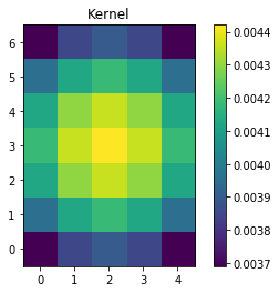
# setup our custom kernel
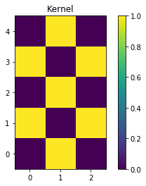
my_kernel = [[0,1,0],[1,0,1],[0,1,0],[1,0,1],[0,1,0]]
# perform convolution
result = ap_convolve(my_arr, my_kernel, normalize_kernel=True, boundary='wrap')
plt.imshow(my_kernel, interpolation='none', origin='lower')
plt.title('Kernel')
plt.colorbar()
plt.show()
fig, axes = plt.subplots(nrows=1, ncols=2)
pmin,pmax = 10, 200
a = axes[0].imshow(my_arr,interpolation='none', origin='lower',vmin=pmin, vmax=pmax)
axes[0].set_title('Before Convolution')
a = axes[1].imshow(result,interpolation='none', origin='lower',vmin=pmin, vmax=pmax)
axes[1].set_title('After Convolution')

fig.subplots_adjust(right = 0.8,left=0)
cbar_ax = fig.add_axes([0.85, 0.15, 0.05, 0.7])
fig.colorbar(a, cax=cbar_ax)
fig.set_size_inches(10,5)
plt.show()
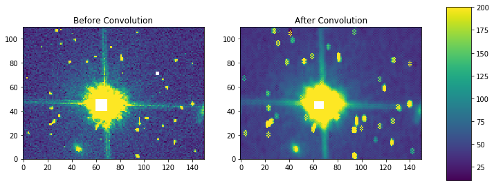
Here is an example using masking with scipy.convolve
# Standard Imports
import numpy as np
from scipy.ndimage import convolve as sp_convolve

# Astronomy Specific Imports
from astropy.io import fits

# Plotting Imports/Setup
import matplotlib.pyplot as plt
%matplotlib inline
# grab subsection of fits images
test_data = './mastDownload/HST/JCZGX1PPQ/jczgx1ppq_flc.fits'
sci1 = fits.getdata(test_data,ext=1)
my_arr = sci1[700:1030,2250:2800]
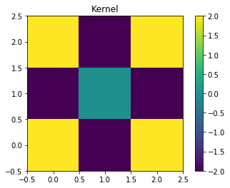
# setup our custom kernel
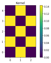
my_kernel = np.array([[0,1,0],[1,0,1],[0,1,0],[1,0,1],[0,1,0]]) * (1/7.0)
# perform convolution
result = sp_convolve(my_arr, my_kernel, mode='wrap')
plt.imshow(my_kernel, interpolation='none', origin='lower')
plt.title('Kernel')
plt.colorbar()
plt.show()
fig, axes = plt.subplots(nrows=1, ncols=2)
pmin,pmax = 10, 200
a = axes[0].imshow(my_arr,interpolation='none', origin='lower',vmin=pmin, vmax=pmax)
axes[0].set_title('Before Convolution')
a = axes[1].imshow(result,interpolation='none', origin='lower',vmin=pmin, vmax=pmax)
axes[1].set_title('After Convolution')

fig.subplots_adjust(right = 0.8,left=0)
cbar_ax = fig.add_axes([0.85, 0.15, 0.05, 0.7])
fig.colorbar(a, cax=cbar_ax)
fig.set_size_inches(10,5)
plt.show()
gauss
Please review the Notes section above before running any examples in this notebook
The gaussian kernel convolution applies a gaussian function convolution to your data array. The Gaussian2DKernel size is defined slightly differently from the IRAF version.
# Standard Imports
import numpy as np

# Astronomy Specific Imports
from astropy.io import fits
from astropy.convolution import convolve as ap_convolve
from astropy.convolution import Gaussian2DKernel
from astroquery.mast import Observations

# Plotting Imports/Setup
import matplotlib.pyplot as plt
%matplotlib inline
# Download test file using astroquery, this only needs to be run once
# and can be skipped if using your own data.
# Astroquery will only download file if not already present.
obsid = '2004663553'
Observations.download_products(obsid,productFilename="jczgx1ppq_flc.fits")
INFO: Found cached file ./mastDownload/HST/JCZGX1PPQ/jczgx1ppq_flc.fits with expected size 167964480. [astroquery.query]
| Local Path | Status | Message | URL |
|---|---|---|---|
| str47 | str8 | object | object |
| ./mastDownload/HST/JCZGX1PPQ/jczgx1ppq_flc.fits | COMPLETE | None | None |
# grab subsection of fits images
test_data = './mastDownload/HST/JCZGX1PPQ/jczgx1ppq_flc.fits'
sci1 = fits.getdata(test_data,ext=1)
my_arr = sci1[700:1030,2250:2800]

# setup our kernel, with 6 sigma and a 3 in x by 5 in y size
gauss_kernel = Gaussian2DKernel(6, x_size=5, y_size=7)
# perform convolution
result = ap_convolve(my_arr, gauss_kernel, normalize_kernel=True)

gauss_kernel
<astropy.convolution.kernels.Gaussian2DKernel at 0x18255efe80>
plt.imshow(gauss_kernel, interpolation='none', origin='lower')
plt.title('Kernel')
plt.colorbar()
plt.show()
fig, axes = plt.subplots(nrows=1, ncols=2)
pmin,pmax = 10, 200
a = axes[0].imshow(my_arr,interpolation='none', origin='lower',vmin=pmin, vmax=pmax)
axes[0].set_title('Before Convolution')
a = axes[1].imshow(result,interpolation='none', origin='lower',vmin=pmin, vmax=pmax)
axes[1].set_title('After Convolution')

fig.subplots_adjust(right = 0.8,left=0)
cbar_ax = fig.add_axes([0.85, 0.15, 0.05, 0.7])
fig.colorbar(a, cax=cbar_ax)
fig.set_size_inches(10,5)
plt.show()

laplace
Please review the Notes section above before running any examples in this notebook
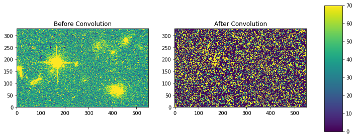
The laplace task runs a image convolution using a laplacian filter with
a subset of footprints. For the scipy.ndimage.filter.laplace
function we will be using, you can feed any footprint in as an array to
create your kernel.
# Standard Imports
import numpy as np
from scipy.ndimage import convolve as sp_convolve
from scipy.ndimage import laplace

# Astronomy Specific Imports
from astropy.io import fits
from astroquery.mast import Observations

# Plotting Imports/Setup
import matplotlib.pyplot as plt
%matplotlib inline
# Download test file using astroquery, this only needs to be run once
# and can be skipped if using your own data.
# Astroquery will only download file if not already present.
obsid = '2004663553'
Observations.download_products(obsid,productFilename="jczgx1ppq_flc.fits")
INFO: Found cached file ./mastDownload/HST/JCZGX1PPQ/jczgx1ppq_flc.fits with expected size 167964480. [astroquery.query]
| Local Path | Status | Message | URL |
|---|---|---|---|
| str47 | str8 | object | object |
| ./mastDownload/HST/JCZGX1PPQ/jczgx1ppq_flc.fits | COMPLETE | None | None |
# grab subsection of fits images
test_data = './mastDownload/HST/JCZGX1PPQ/jczgx1ppq_flc.fits'
sci1 = fits.getdata(test_data,ext=1)
my_arr = sci1[700:1030,2250:2800]

# setup our laplace kernel with a target footprint (diagonals in IRAF)
footprint = np.array([[0, 1, 0], [1, 1, 1], [0, 1, 0]])
laplace_kernel = laplace(footprint)
# perform scipy convolution
result = sp_convolve(my_arr, laplace_kernel)
plt.imshow(laplace_kernel, interpolation='none', origin='lower')
plt.title('Kernel')
plt.colorbar()
plt.show()
fig, axes = plt.subplots(nrows=1, ncols=2)
a = axes[0].imshow(my_arr,interpolation='none', origin='lower',vmin=0, vmax=70)
axes[0].set_title('Before Convolution')
a = axes[1].imshow(result,interpolation='none', origin='lower',vmin=0, vmax=70)
axes[1].set_title('After Convolution')

fig.subplots_adjust(right = 0.8,left=0)
cbar_ax = fig.add_axes([0.85, 0.15, 0.05, 0.7])
fig.colorbar(a, cax=cbar_ax)
fig.set_size_inches(10,5)
plt.show()
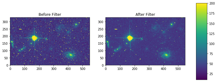
median-rmedian
Please review the Notes section above before running any examples in this notebook
Apply a median filter to your data array, and save the smoothed image
back out to a FITS file. We will use the
scipy.ndimage.filters.median_filter function.
# Standard Imports
import numpy as np
from scipy.ndimage.filters import median_filter

# Astronomy Specific Imports
from astropy.io import fits
from astroquery.mast import Observations

# Plotting Imports/Setup
import matplotlib.pyplot as plt
%matplotlib inline
# Download test file using astroquery, this only needs to be run once
# and can be skipped if using your own data.
# Astroquery will only download file if not already present.
obsid = '2004663553'
Observations.download_products(obsid,productFilename="jczgx1ppq_flc.fits")
INFO: Found cached file ./mastDownload/HST/JCZGX1PPQ/jczgx1ppq_flc.fits with expected size 167964480. [astroquery.query]
| Local Path | Status | Message | URL |
|---|---|---|---|
| str47 | str8 | object | object |
| ./mastDownload/HST/JCZGX1PPQ/jczgx1ppq_flc.fits | COMPLETE | None | None |
# create test array
test_data = './mastDownload/HST/JCZGX1PPQ/jczgx1ppq_flc.fits'
out_file = 'median_out.fits'
sci1 = fits.getdata(test_data,ext=1)
my_arr = sci1[700:1030,2250:2800]

# apply median filter
filtered = median_filter(my_arr,size=(3,4))
# save smoothed image to a new FITS file
hdu = fits.PrimaryHDU(filtered)
hdu.writeto(out_file, overwrite=True)
fig, axes = plt.subplots(nrows=1, ncols=2)
pmin,pmax = 10, 200
a = axes[0].imshow(my_arr,interpolation='none', origin='lower',vmin=pmin, vmax=pmax)
axes[0].set_title('Before Filter')
a = axes[1].imshow(filtered,interpolation='none', origin='lower',vmin=pmin, vmax=pmax)
axes[1].set_title('After Filter')

fig.subplots_adjust(right = 0.8,left=0)
cbar_ax = fig.add_axes([0.85, 0.15, 0.05, 0.7])
fig.colorbar(a, cax=cbar_ax)
fig.set_size_inches(10,5)
plt.show()
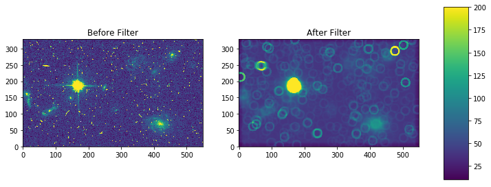
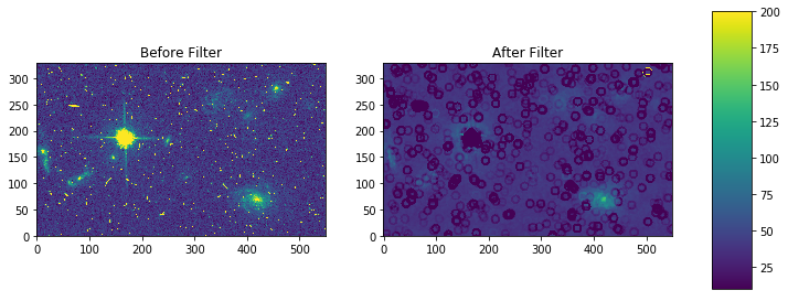
For a ring median filter we can supply a more specific footprint to the
median_filter function. You can easily generate this footprint using
the astropy.convolution library. In this example we will also show
how to use the equivalent of the IRAF zloreject/zhireject parameter. The
handling of numpy nan values is only available with the
Astropy convolution.
# Standard Imports
import numpy as np

# Astronomy Specific Imports
from astropy.io import fits
from astropy.convolution import convolve as ap_convolve
from astropy.convolution import Ring2DKernel

# Plotting Imports/Setup
import matplotlib.pyplot as plt
%matplotlib inline
# create test array
test_data = './mastDownload/HST/JCZGX1PPQ/jczgx1ppq_flc.fits'
sci1 = fits.getdata(test_data,ext=1)
my_arr = sci1[700:1030,2250:2800]

# create ring filter
ringKernel = Ring2DKernel(10,5)

# apply a zloreject value by setting certain values to numpy nan
my_arr[my_arr < -99] = np.nan

# apply median filter
filtered = ap_convolve(my_arr, ringKernel, normalize_kernel=True)
plt.imshow(ringKernel, interpolation='none', origin='lower')
plt.title('Ring Footprint')
plt.colorbar()
plt.show()

fig, axes = plt.subplots(nrows=1, ncols=2)
pmin,pmax = 10, 200
a = axes[0].imshow(my_arr,interpolation='none', origin='lower',vmin=pmin, vmax=pmax)
axes[0].set_title('Before Filter')
a = axes[1].imshow(filtered,interpolation='none', origin='lower',vmin=pmin, vmax=pmax)
axes[1].set_title('After Filter')

fig.subplots_adjust(right = 0.8,left=0)
cbar_ax = fig.add_axes([0.85, 0.15, 0.05, 0.7])
fig.colorbar(a, cax=cbar_ax)
fig.set_size_inches(10,5)
plt.show()
mode-rmode
Please review the Notes section above before running any examples in this notebook
The mode calculation equation used in the mode and rmode IRAF tasks (3.0*median - 2.0*mean) can be recreated using the scipy.ndimage.generic_filter function. The equation was used as an approximation for a mode calculation.
# Standard Imports
import numpy as np
from scipy.ndimage import generic_filter

# Astronomy Specific Imports
from astropy.io import fits
from astroquery.mast import Observations

# Plotting Imports/Setup
import matplotlib.pyplot as plt
%matplotlib inline
# Download test file using astroquery, this only needs to be run once
# and can be skipped if using your own data.
# Astroquery will only download file if not already present.
obsid = '2004663553'
Observations.download_products(obsid,productFilename="jczgx1ppq_flc.fits")
INFO: Found cached file ./mastDownload/HST/JCZGX1PPQ/jczgx1ppq_flc.fits with expected size 167964480. [astroquery.query]
| Local Path | Status | Message | URL |
|---|---|---|---|
| str47 | str8 | object | object |
| ./mastDownload/HST/JCZGX1PPQ/jczgx1ppq_flc.fits | COMPLETE | None | None |
def mode_func(in_arr):
    f = 3.0*np.median(in_arr) - 2.0*np.mean(in_arr)
    return f
For a box footprint:
# create test array
test_data = './mastDownload/HST/JCZGX1PPQ/jczgx1ppq_flc.fits'
sci1 = fits.getdata(test_data,ext=1)
my_arr = sci1[700:1030,2250:2800]

# apply mode filter
filtered = generic_filter(my_arr, mode_func, size=5)
fig, axes = plt.subplots(nrows=1, ncols=2)
pmin,pmax = 10, 200
a = axes[0].imshow(my_arr,interpolation='none', origin='lower',vmin=pmin, vmax=pmax)
axes[0].set_title('Before Filter')
a = axes[1].imshow(filtered,interpolation='none', origin='lower',vmin=pmin, vmax=pmax)
axes[1].set_title('After Filter')

fig.subplots_adjust(right = 0.8,left=0)
cbar_ax = fig.add_axes([0.85, 0.15, 0.05, 0.7])
fig.colorbar(a, cax=cbar_ax)
fig.set_size_inches(10,5)
plt.show()
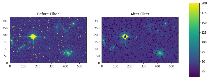
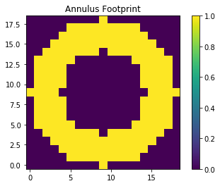
For a ring footprint (similar to IRAF’s rmode):
# Standard Imports
import numpy as np
from scipy.ndimage import generic_filter

# Astronomy Specific Imports
from astropy.io import fits
from astroimtools import circular_annulus_footprint

# Plotting Imports/Setup
import matplotlib.pyplot as plt
%matplotlib inline
# create test array
test_data = './mastDownload/HST/JCZGX1PPQ/jczgx1ppq_flc.fits'
sci1 = fits.getdata(test_data,ext=1)
my_arr = sci1[700:1030,2250:2800]

# create annulus filter
fp = circular_annulus_footprint(5, 9)
# apply mode filter
filtered = generic_filter(my_arr, mode_func, footprint=fp)
plt.imshow(fp, interpolation='none', origin='lower')
plt.title('Annulus Footprint')
plt.colorbar()
plt.show()
fig, axes = plt.subplots(nrows=1, ncols=2)
pmin,pmax = 10, 200
a = axes[0].imshow(my_arr,interpolation='none', origin='lower',vmin=pmin, vmax=pmax)
axes[0].set_title('Before Filter')
a = axes[1].imshow(filtered,interpolation='none', origin='lower',vmin=pmin, vmax=pmax)
axes[1].set_title('After Filter')

fig.subplots_adjust(right = 0.8,left=0)
cbar_ax = fig.add_axes([0.85, 0.15, 0.05, 0.7])
fig.colorbar(a, cax=cbar_ax)
fig.set_size_inches(10,5)
plt.show()
Not Replacing
runmed - see images.imutil.imsum
fmode - see images.imfilter.mode
fmedian - see images.imfilter.median
gradient - may replace in future